To the Basics: Bayesian Inference on A Binomial Proportion

Think of something observable - countable - that you care about with only one outcome or another.

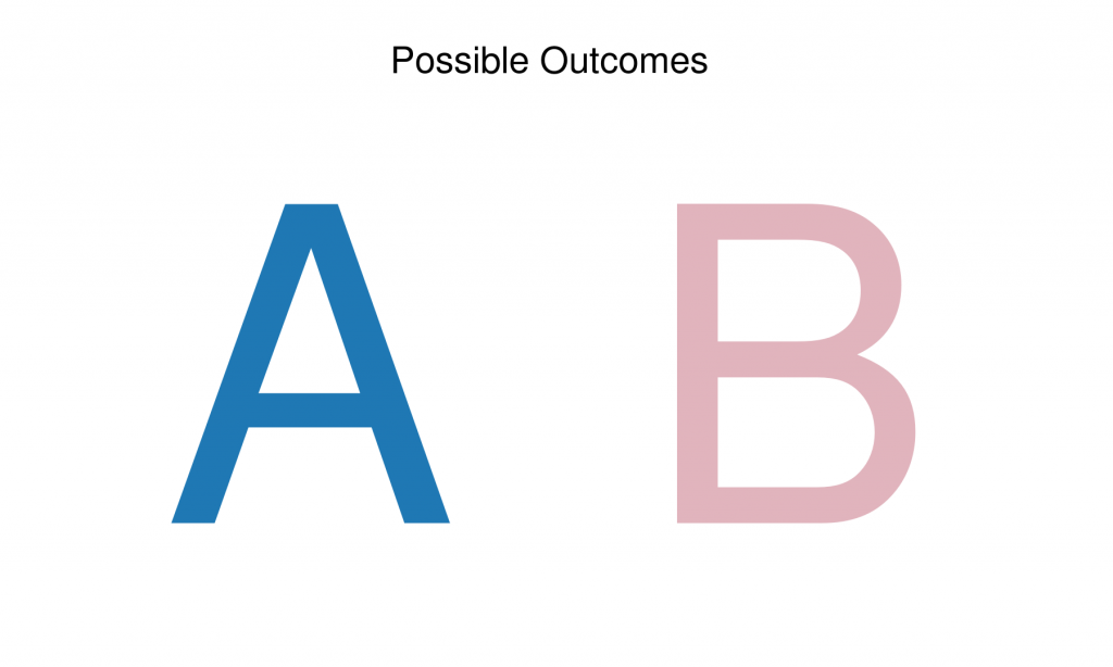
It could be the votes cast in a two-way election in your town, or the free throw shots the center on your favorite basketball team takes, the survival of the people diagnosed with a specific form of cancer after five years, all the red/black bets ever placed on a specific roulette wheel, the gender of all the children in 18th century France; many phenomena in the world either fit this discription or can be thought of in this way. The most important thing is that the outcome of this phenomenon - or the way you group the outcomes - can only take one of two values: $A$ or $B$:

Let's call this phenomenon $Z$.

Let's also define a number, $N$, as the total number of occurances of $Z$. So it is the total number of shots taken, the total count of people diagnosed, the total number of votes cast.

Now remember, $Z$ is something you care about. It is likely, since you care so much about $Z$, that you have some preference for one of the two possible outcomes. For the purposes of this example, let's say we prefer $A$. $A$ is a shot made, a vote recieved, a survival. $A$ is a "success", from your perspective. And an outcome of $B$ is a failure.

Lets define another value, given that we prefer $A$ outcomes over $B$ outcomes. $Y$ is the number of $A$ outcomes out of all the times $N$ happens. It is the number of votes that your candidate is going to get in that election, the number of free throws the big man makes, the number of cancer patients who survive.

Of course, we can define this kind of process in this way even if we don't actually prefer one outcome over the other. In the case of the gender of newborns, for instance: we can define $A$ as the birth of a girl and $B$ as the birth of a boy, and treat the birth of a boy as a failure, just for the purposes of our model and not because all little boys are born clinically insane.

You, as a keen, long-time observer of $Z$, probably have some opinion on the share of $A$ outcomes in the total of all occurrences of $Z$ that you likely express as an opinion on the value of the ratio of $A$ outcomes to all occurances of $Z$, or $Y/N$, e.g.:

• More often than not, $Z$ equals $B$ or $Y/N < 0.5$
• Most of the time, $Z$ equal $A$ or $Y/N > 0.5$
• $Z$ is as likely to equal $A$ as it is to equal $B$ or $Y/N = 0.5$

It would be nice, probably, to have an actual number as an estimate for $Y/N$, or perhaps a range of numbers you can be confident contains the value of $Y/N$.

And perhaps you want to make some prediction about future occurances of $Z$. You want to know if someone you know with that particular form of cancer is likely to still be alive five years from now.

Or maybe your friend, also a fan of that same basketball team, thinks that your guy actually only misses about half the time. Or a political talking head says that  your candidate is going to lose big. You probably want a way to compare your beliefs with theirs.

Essentially, we would like to estimate the unknown quantity $\theta$, preferably with some additional estimate of our uncertainty of this value, use that estimate to predict future values of trials of $Z$, and, given that estimate, get an idea of who is more likely right about that quantity given disagreements.

Translating our above situation into the language of probability, this phenomenon $Z$ - any phenomenon with a ``this'' or ``that'' outcome - can be modeled mathematically as a ``random variable'' $Y$, with a binomial probability distribution:

$p(Y) = {N \choose Y} \theta^Y (1-\theta)^{(N-Y)}$

where $N$ is number of trials - the total number of cancer patients, shots taken, votes cast - $Y$ is the number of successes or cases where the outcome equals A, and $\theta$ is that unknown value between 0 and 1 that equals the proportion $Y/N$. This distribution describes the probability that $Z$ equals $A$ $Y$ times in $N$  occurances (also called trials) of $Z$.

$Z$ can also be modeled as the product of $N$ individual occurances of $Y$, $y_i$, where $y_i$ equals 1 if the outcome equals A and 0 if the outcome equals B, and  $\theta$ is still the unknown proportion of A outcomes in all occurances of $Y$:

$p(z_i=A) = p(y_i)$

$p(y_i) = \theta^{y_i} (1-\theta)^{(1-y_i)}$

This formulation - really a special case of the binomial distribution where N equals 1 - is often refered to a bernoulli random variable. The product of $N$ individual occurances - $y_1, y_2, y_3, ..., y_N$- is also equal to the conditional probability of the total number of successes Y on the value of $\theta$, because the probability of a number of independent events occuring together is the product of all of their individual probabilities:

$p(Y) = \Pi_{i=1}^{N} \theta^{y_i} (1-\theta)^{(1-y_i)}$

And in fact this product simplifies to the formula for the binomial distribution above.

It is important to realize that the value most useful for us to know the most about in the formulas above is not $N$ or $Y$ or any single $y_i$ but $\theta$.

To illustrate all of this further, I'm going to let R simulate an ``true'', unknown $\theta$ or $Y/N$ and hide that value from myself as a fixed quantity $\theta_{true}$:

That function call generates a single pseudo-random number between 0 and 1 from a uniform distribution, meaning that the value is equally as likely to be anywhere in that (0,1) interval.

I'm going to use that hidden proportion to generate a ``true population'' Z, with an unknown N total number of occurances, distributed according to our hidden $\theta_{true}$:

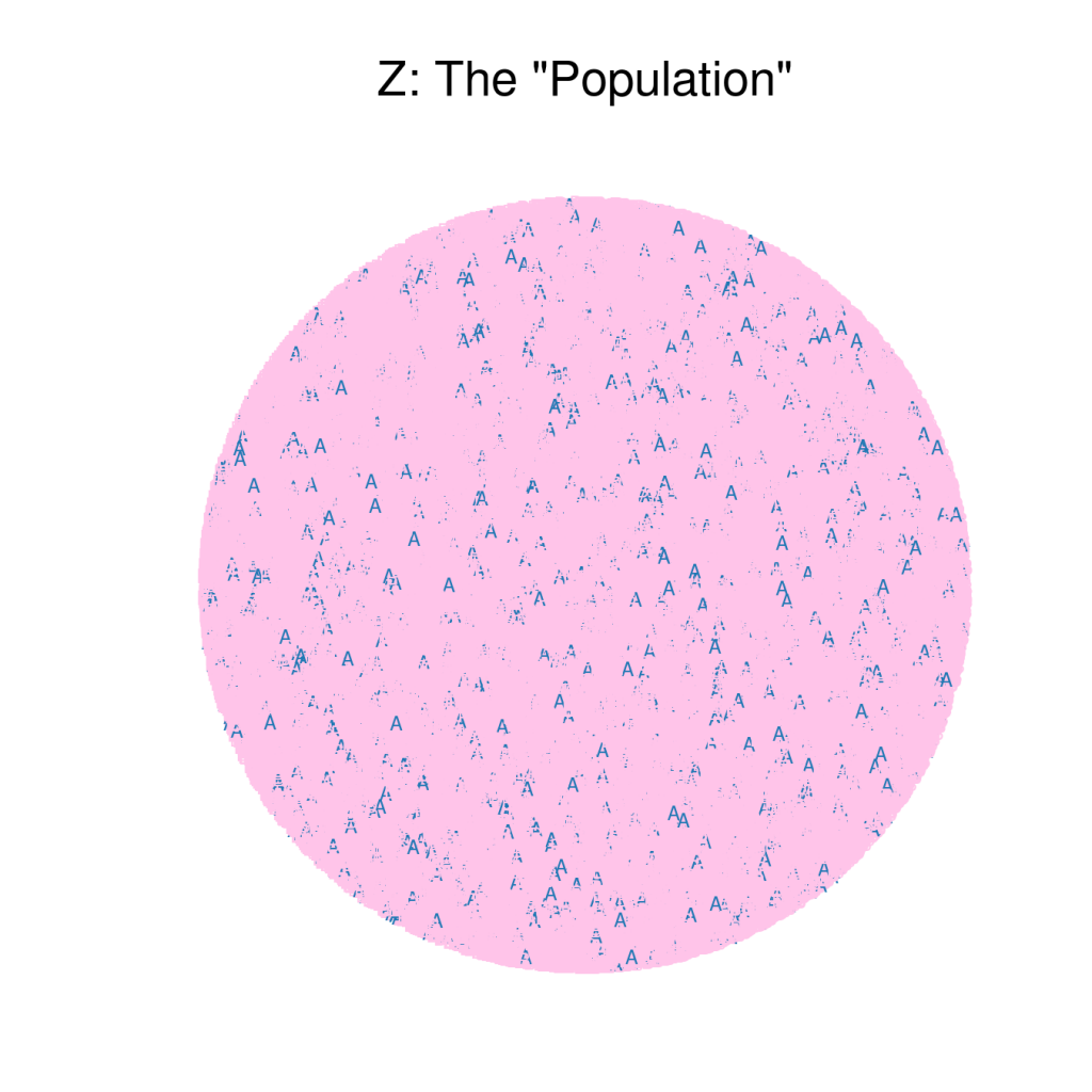
Since Z is very large, and we are pretending it is not data in memory on my computer but a set of outcomes that are very difficult or impossible to count in their entireity, we will be working with a sample pulled from Z, some small subset that we can count and infer something about the value of $\theta_{true}$ from. But as I said above, we know something about Z already. We follow Z very closely. We talk to everyone we know about the election, even if we don't keep a running tally of who they say they're voting for. We watch every game, even if we don't have an exact count of shots missed vs shots made. We have some prior understanding of Z already. Of course, most of the time, our first prior looks something like this:

I can't calculate $\theta_{true}$ from that understanding, at least not just by looking at it. It probably wouldn't be possible to count all the $A$ outcomes up there, given how jumbled they are, and even if it was, there's no way I can count them in any reasonable time. Maybe most of them haven't even happened yet, in which case I definitely can't count them. Actually, I don't even know what the total value of N is.

But I can tell some things from that picture, right? For instance, I know that there are definitely at least some trials where the outcome of $Z$ is $A$. I know that there are at least some trials where the outcome of $Z$ is $B$. In this case, actually, $A$ outcomes look pretty rare and it seems a pretty safe bet to say even more than that: our boy misses most of his free throws, or our guy is going to lose this election.

Lets get our sample, which we will call $N_{samp}$, from our population:

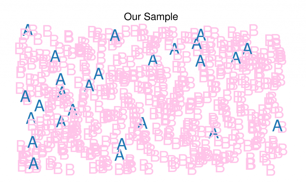
In this case, we were able to obtain a sample of 500 trials of Z, and they look, before we do anything to them, like this:

Since our random variable stores $A$ outcomes as successes or 1's and $B$ outcomes as failures or 0's, we can easily obtain our sample $Y$ - $Y_{samp}$ by summing up all our $N_{samp}$ occurances of $Z$.

Which in this case turns out to be 26.

We could just calculate the sample proportion of $Y_{samp}/N_{samp}$ and take that for our estimate of $\theta_{true}$. In this case, that would be 0.052.

But that estimate only allows us to achieve part of one of our three goals above. We can't really compare our opinions to anyone elses with any meaning, and we can't use that number by itself to predict future values.

But what if we treat our $\theta = Y/N$ parameter as a random variable? What if we assign it a 'mean' or a most likely value, and a variance, or some quantification of uncertainty around that mean?

If we have probability distributions for all of our values of interest, we can use Bayes theorem:

$p(Y_{samp},N_{samp},\theta_{true}) = p(Y_{samp},N_{samp}|\theta_{true}) p(\theta_{true})$

$p(\theta_{true},Y_{samp},N_{samp}) = p(\theta_{true}|Y_{samp}) p(Y_{samp})$

$p(Y_{samp},\theta_{true}) = p(\theta_{true},Y_{samp})$

$p(Y_{samp},N_{samp}|\theta_{true}) p(\theta_{true}) = p(\theta_{true}|Y_{samp},N_{samp}) p(Y_{samp},N_{samp})$

$p(\theta_{true}|Y_{samp},N_{samp}) = \frac{p(Y_{samp},N_{samp}|\theta_{true}) p(\theta_{true})}{p(Y_{samp},N_{samp})}$

In this case, the posterior probabilility is the conditional probability distribution we get for $\theta_{true}$ given the data $Y,N$ and our prior distribution for $\theta_{true}$.

The generalization of Bayes' theorem for use in inference involving the entire probability distribution of a random variable instead of just a point estimate of a probability allows us to, in essence, ignore the term $p(Y_{samp},N_{samp})$ in the expression:

$p(\theta_{true}|Y_{samp},N_{samp}) = \frac{p(Y_{samp},N_{samp}|\theta_{true}) p(\theta_{true})}{p(Y_{samp},N_{samp})}$

because we know that it, with respect to the conditional distribution of $\theta$ - $p(\theta_{true}|Y_{samp},N_{samp})$ - is just a constant. And since $p(\theta_{true}|Y_{samp},N_{samp})$ is a probability distribution, we know that it has to integrate to 1 in the end, so determining that normalizing constant after we have the non-normalized distribution shouldn't be a problem.

This allows us to work with the proportional relationship, giving us our model:

$p(\theta_{true}|Y_{samp},N_{samp}) \propto p(\theta_{true}) p(Y_{samp},N_{samp}|\theta_{true})$

or:

The posterior is proportional to the product of the prior and the likelihood.

This is the central - really the only - tool of Bayesian statistical inference. And it suggests one of the central appeals, to me, of the approach: every input into a Bayesian framework is expressed as probability and every output of a Bayesian framework is expressed as probability.

To use this generalization of Bayes' theorem to answer our above questions, we first need to come up with a model for $\theta_{true}$'s distribution. There are a number of ways that $\theta_{true}$ could be distributed. In fact, any distribution that ensures that the value of $\theta_{true}$ will be between 0 and 1 will do.

In this first example, we will take advantage of the fact that there exists aconjugateprior for the binomial distribution: the beta distribution.

The beta distribution

$p(\theta) = \theta^{\alpha-1} (1-\theta)^{\beta-1}$

looks very similar in form to the binomial distribution

$p(Y) = {N \choose Y} \theta^Y (1-\theta)^{(N-Y)}$

except it represents the probabilities assigned to values of $\theta$ in the domain $(0,1)$ given values for the parameters $\alpha$ and $\beta$, as opposed to the binomial distribution above, which represents the probability of values of $Y$ given $\theta$.

The concept of conjugacy is fairly simple. It just means that the functional forms of the distributions of which you are calculating the product are the same, so they multiply easily. The product of a beta and a binomial, given their identical functional forms, is simply:

$\theta^{\alpha-1} (1-\theta)^{\beta-1} * {N \choose Y} \theta^Y (1-\theta)^{(N-Y)} = {N \choose Y} \theta^{(Y+\alpha-1)} (1-\theta)^{(N-Y+\beta-1)}$

and since ${N \choose Y}$ is just a constant in relationship to $\theta$, our final Bayes formulation of our beta prior, binomial likelihood model is:

$p(\theta_{true}|Y_{samp},N_{samp}) \propto \theta^{(Y+\alpha-1)} (1-\theta)^{(N-Y+\beta-1)}$

This also is a beta probability distribution, with $\alpha_{posterior}$ equal to $Y+\alpha_{prior}$ and $\beta_{posterior}$ equal to $N-Y+\beta_{prior}$.

But how do we choose our beta priors?

The shape of a beta distribution is dictated by the values of those $\alpha$ and $\beta$ parameters and shifting those values can allow you to represent a wide range of different prior beliefs about the distribution of $\theta$. Priors can be ``uninformative'' or ``informative'', meaning we can weight our prior probabilities very low in relationship to the data or we can weight them higher, informing our outcome - the posterior - more as we weight them more.

A simple function - using ggplot2's qplot - to examine different values of $\alpha$ and $\beta$ and their effect on the shape of the distribution allows us to show this:

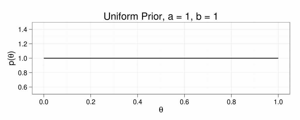
Setting $\alpha$ and $\beta$ both equal to 1 gives us an non-informative uniform prior, allowing us to express that we believe $\theta_{true}$ could be anywhere in the interval $(0,1)$ with equal probability, meaning that the proportion of successes to failures - A outcomes to B outcomes - could be anything:

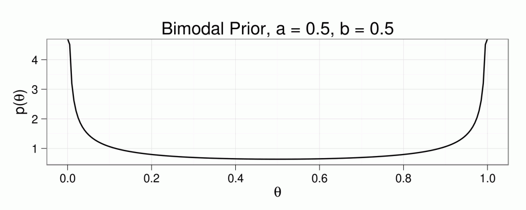
Setting $\alpha$ and $\beta$ both equal to 0.5 gives us an weakly informative uniform prior that expresses a belief that $\theta_{true}$ is more likely to be at either extreme end of the distribution than anywhere in the center of it, meaning it is more likely that we get all successes or all failures than it is we get some more even mixture of outcomes:

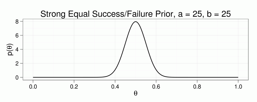
Setting $\alpha$ and $\beta$ both equal to a high value gives us an more strongly informative prior expressing that we believe that $\theta_{true}$ is likely to be at the center or that it is equally likely to see successes and failures:

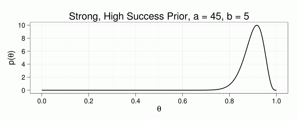
We could express a stronger belief that $\theta_{true}$ is high - that success is very likely - with a higher $\alpha$ and a lower $\beta$:

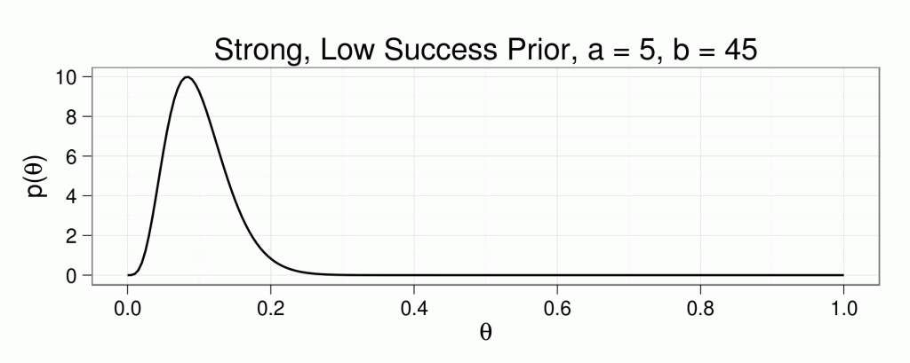
or a stronger belief that $\theta_{true}$ is very low - that success is unlikely - with a lower $\alpha$ and a higher $\beta$:

Essentially, higher values of the ratio of $\alpha$ to $\beta$ weights higher values of $\theta$ higher, lower values of that ratio place greater weight on lower $\theta$ values, and higher value of $\alpha + \beta$ indicates higher certainty.

Still, choosing these $\alpha$'s and $\beta$'s may seem a bit arbitrary. Perhaps a more intuitive way to choose an informative prior is to allow ourselves the ability to calculate analogous values to $\theta_{true}$ and $N$ - essentially a value that actually quantifies our prior belief about the likelihood of success and a value that quantifies how strongly we weigh that belief as a prior ``sample size''. We want to be able to express the 'mean' of our prior distribution - its most likely value - and something like a variance or how tightly clustered it is around that mean.

The mean of a beta distribution is:

$m = \frac{\alpha}{\alpha + \beta}$

and the ``sample size'' $n$ is:

$n = \alpha + \beta$

and solving those two equations for $\alpha$ and $\beta$ gives us

$\alpha = n * m$
$\beta = n * (1 - m)$

where, again, $n$ expresses how large our prior ``sample size'' is - i.e. the higher it is, the stronger our beliefs - and $m$ expresses our actual prior belief for the value of $\theta_{true}$.

Getting the values for our prior distribution using any chosen values for $m$ and $n$ can be acomplished with a simple R function:

And expressing the likelihood - a binomial - as a beta where $\alpha$ equals $Y + 1$ and $\beta$ equals $N - Y + 1$ is another simple function.

And combining them into the posterior beta distribution:

and getting the mean:

the mode:

and the standard deviation of the posterior:

can all be accomplished using functions of similar structure.

First, we generate a model with a uniform prior:

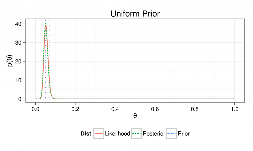
where the dotted gray lines indicate the outer bounds of our credibility interval and the dotted blue line indicates our mean.

The mean of our posterior distribution equals 0.052, the mode equals 0.05, and the standard deviation equals 0.01.

This gives us a 95% (normal-approximation) credibility interval of 0.033 to 0.071.

Our posterior and our likelihood distributions are almost identical, as would be expected, since our prior is essentially that we have no idea and the data should give us all of the information in our posterior.

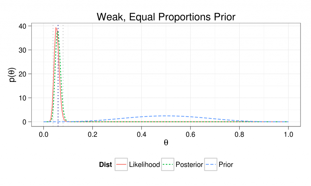
A weak, equal probability prior gives:

The mean of our posterior distribution equals 0.059, the mode equals 0.057, and the standard deviation equals 0.01.

This gives us a 95% (normal-approximation) credibility interval of 0.039 to 0.08.

Our mean and mode is a bit higher than before, as we weighted our prior beliefs a little bit, but our posterior is very close to our likelihood, meaning that most of the result was informed by the data.

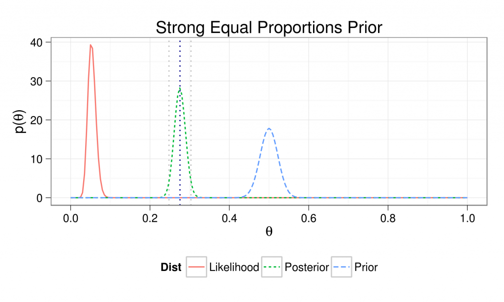
A strong equal prior gives:

The mean of our posterior distribution equals 0.276, the mode equals 0.275, and the standard deviation equals 0.014.

This gives us a 95% (normal-approximation) credibility interval of 0.248 to 0.303.

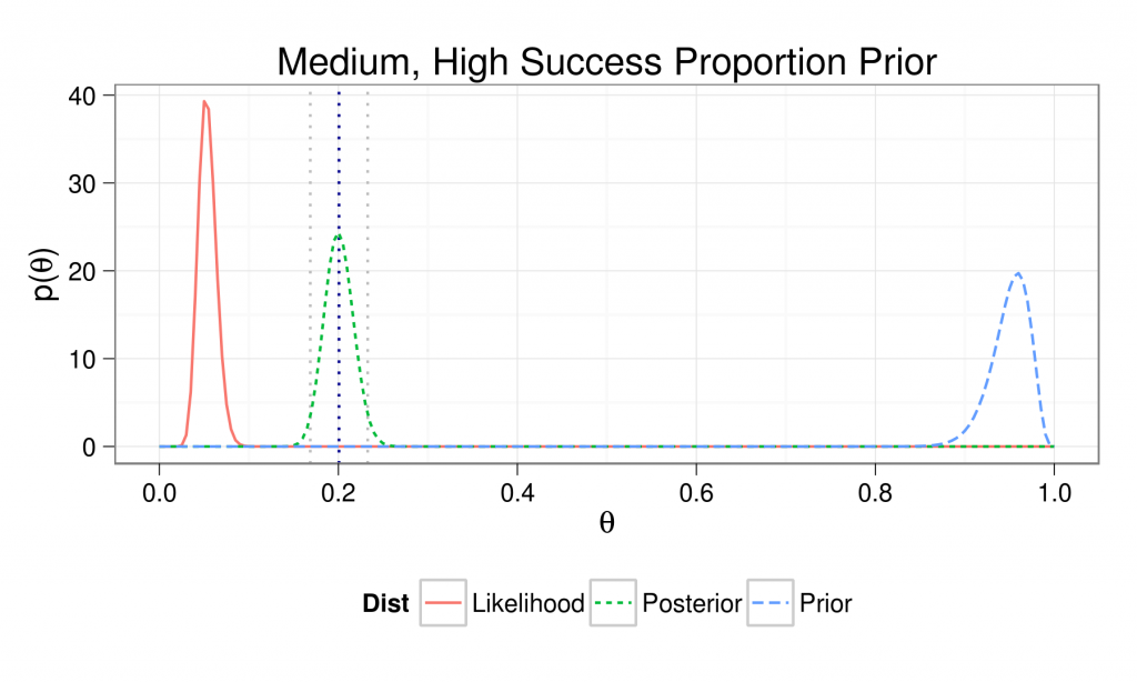
A model with a medium, high success prior looks like:

The mean of our posterior distribution equals 0.201, the mode equals 0.2, and the standard deviation equals 0.016.

This gives us a 95% (normal-approximation) credibility interval of 0.169 to 0.233.

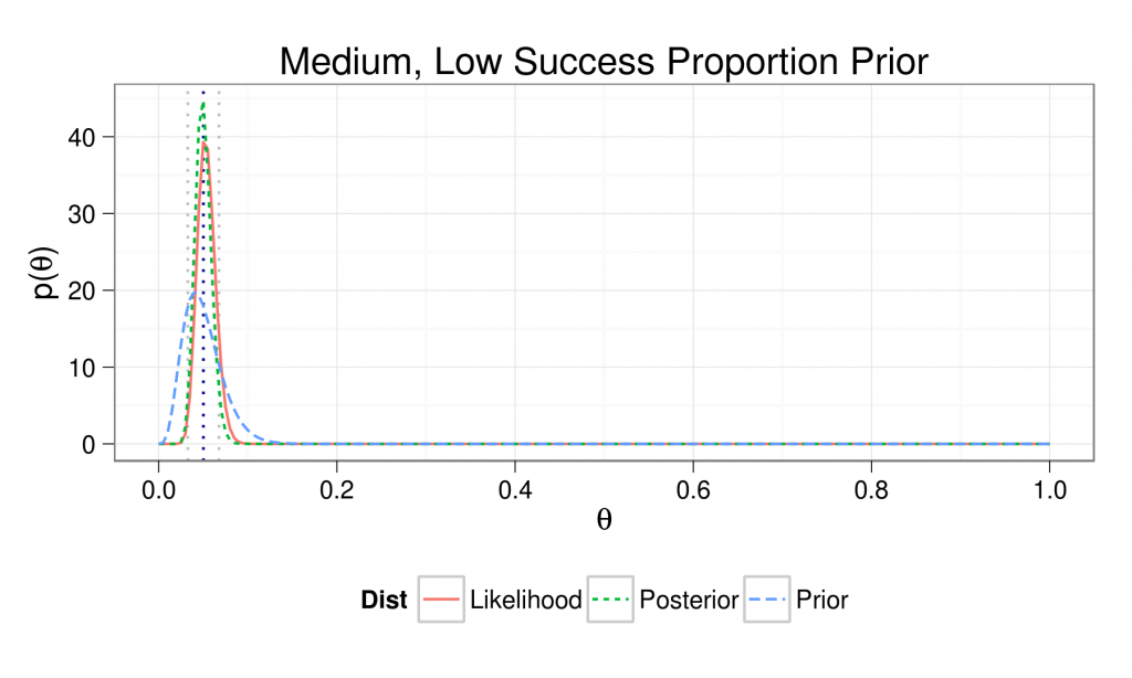
And finally a medium, low success proportion prior:

The mean of our posterior distribution equals 0.05, the mode equals 0.049, and the standard deviation equals 0.009.

This gives us a 95% (normal-approximation) credibility interval of 0.033 to 0.068.

So how did each of our models do, in this case? Well, since we simulated this data, we can discover that $\theta_{true}$ actually equals 0.042, or about 4% of all occurances of $Z$ result in $A$ outcomes.

The results of all of our models are:

 

	Mean of Dist	Mode of Dist	Std Dev of Dist
Uniform Prior	0.052	0.050	0.010
Weak, Equal Proportions	0.059	0.057	0.010
Strong, Equal Proportions	0.276	0.275	0.014
Medium, High Success	0.201	0.200	0.016
Medium, Low Success	0.050	0.049	0.009

 

And it is obvious that our two initial priors - the non-informative uniform and the weakly informative equal proportions - and our last prior - the medium confidence of a low proportion of success outcomes - all gave fairly accurate estimates of $\theta_{true}$.

Our strong, equal proportions prior and medium, high sucess prior - what could be called, with a terminology nod to John Myles White, our "strong, wrong" priors - gave pretty bad estimates, obviously, though the likelihood moved our posterior much closer to the truth in the second case, and our updated belief is much better in both cases than where we started.

This susceptability to strong, wrong priors is a common critique of Bayesian inference. But these results aren't incorrect, are they? My results in the cases of my strong, wrong priors are the correct highest probability distributions of $\theta_{true}$ conditional on my incorrect priors. But I would be an idiot to choose those priors, given what I already know about $\theta$, which is, remember:

And if I didn't know anything about $\theta_{true}$ or I had an idea but not a lot of confidence in it, why wouldn't I choose either of my first two priors, both of which arrived at perfectly serviceable estimates for $\theta_{true}$?

As importantly, in both my strong, wrong priors, my assumptions are clearly stated and easy to interpret and critique. If I published something using those assumptions, and everyone and their mother could just look out and see that:

It would be easy to establish that my analysis was based on those flawed assumptions. It could even be done by someone who has only a cursory understanding of how I actually arrived at those estimates.

In future posts, I would like to continue this example and examine the effects of smaller sample sizes and the ease of updating beliefs using a series of smaller samples, much as Kruschke and Bolstadt do in their texts. I think their choices for visualizations and some of the explanations in Bolstadt are sometimes more confusing than necessary, and establishing a stronger single thread through the explanations would make things more intuitive, so I'm going to attempt to actually do that here. Krushke and Gelman have excellent explanations for all of this that are well worth the read. I would also like to look at comparing beliefs and predicting future values in binomial proportions as well.

At his seminar on Bayesian methods back in April, John Myles White said something about traditional statisticians being better at actually getting things done over the course of the development of modern statistics. I didn't really understand what he meant until recently.

The basic toolkit of Bayesian statistics produces intuitive, easier to understand - and use and update and compare - outputs through comparatively difficult computational and mathematical procedures. Everything in and out of a Bayesian analysis is probability and can be combined or broken apart according to the rules of probability. But understanding code and sampling algorithms - really understanding algorithms and computation generally - and a much deeper grasp of probability distribution theory are much more important in understanding Bayesian inference much earlier on.

Basic traditional statistical methods produce output that is fairly difficult to understand through comparatively simple computational and mathematical procedures. Most results in traditional statistics depend on logical appeals to unseen - really un-see-able - asymptotic properties of the estimators being used and assumptions and relationships between samples and populations that may be valid or not in any given case.

This is a very real catch-22: always easier to understand and use, much harder to do initially versus always harder to understand and use, much easier to do initially. I think that much of the difficulty so many have when faced with statistics comes from the fact that traditional OUTPUTS are so unintuitive and seem to exist in isolation or only in relationship to something with a touch of the `other' about it.

The concept of maximum likelihood and the MLE methods that comprise the basis of much of traditional methods are very elegant - actually quite beautiful - logical constructs that manage to give one the ability to say SOMETHING when faced with the problem of lots of data and not a lot of computational power.

But that's not our problem anymore. Now we have lots of data AND lots of computational power. Our problem now is statistical literacy, and building on the body of human knowledge in a way that is both rigorous and democratic.

Credit where credit is due: I've studied and digested the work of the following to learn this stuff and everything I'm going to post here and much of what I use on a daily basis in my work:

• Hadley Wickam's ggplot2 - this R package is something of an obsession of mine. Learn it well and essentially any static visualization is available to you. Incredibly powerful tool.
• Scott Lynch's Introduction to Applied Bayesian Statistics and Estimation for Social Scientists - This book wasn't on my original list, but it has become my first stop. Especially if you think in code instead of equations, his explanations are fantastic and his walkthroughs of sampling algorithms and MCMC are great. It can be purchased here.

and of course the Bolstadt, Kruschke and Gelman books and the work of John Myles White mentioned in my initial post here.